Ejemplo SVM empresas en re organización#
import pandas as pd
import numpy as np
import matplotlib.pyplot as plt
import matplotlib.ticker as mtick
import seaborn as sns
from sklearn.model_selection import train_test_split
from sklearn.svm import SVC
from sklearn.preprocessing import StandardScaler
from sklearn.metrics import classification_report, confusion_matrix, roc_auc_score, roc_curve
from sklearn.metrics import ConfusionMatrixDisplay, precision_score, precision_recall_curve, recall_score, accuracy_score, f1_score
path = "BD empresas en re organización.xlsx"

xls = pd.ExcelFile(path)

df = pd.read_excel(path, sheet_name=xls.sheet_names[0])

df.head()
| Razón Social | Margen EBIT | Carga financiera | Margen neto | CxC | CxP | Solvencia | Apalancamiento | En Reorganización | |
|---|---|---|---|---|---|---|---|---|---|
| 0 | AACER SAS | 0.071690 | 0.000000 | 0.042876 | 0.104095 | 0.153192 | 1.877078 | 1.642505 | 0 |
| 1 | ABARROTES EL ROMPOY SAS | 0.017816 | 0.000000 | 0.010767 | 0.018414 | 0.000000 | 0.000000 | 0.865044 | 0 |
| 2 | ABASTECIMIENTOS INDUSTRIALES SAS | 0.144646 | 0.054226 | 0.059784 | 0.227215 | 0.025591 | 1.077412 | 1.272299 | 0 |
| 3 | ACME LEON PLASTICOS SAS | 0.004465 | 0.000000 | -0.013995 | 0.073186 | 0.127866 | 0.000000 | 1.391645 | 0 |
| 4 | ADVANCED PRODUCTS COLOMBIA SAS | 0.141829 | 0.050810 | 0.053776 | 0.398755 | 0.147678 | 0.675073 | 2.118774 | 0 |
# Conteo absoluto
conteo_clases = df['En Reorganización'].value_counts()
# Porcentaje
porcentaje_clases = df['En Reorganización'].value_counts(normalize=True) * 100

# Mostrar conteo y porcentaje
print("Cantidad de empresas por clase:")
print(conteo_clases)
print("\nPorcentaje de empresas por clase:")
print(porcentaje_clases.round(2))
Cantidad de empresas por clase:
En Reorganización
1    342
0    287
Name: count, dtype: int64

Porcentaje de empresas por clase:
En Reorganización
1    54.37
0    45.63
Name: proportion, dtype: float64
SVM:#
# ------------------------
# Selección de variables
# ------------------------
variables_seleccionadas = ['Margen EBIT',
                           'Carga financiera',
                           'Margen neto',
                           'CxC',
                           'CxP',
                           'Solvencia',
                           'Apalancamiento']

# Variable objetivo
target = 'En Reorganización'

# ------------------------
# Preparar datos
# ------------------------
X = df[variables_seleccionadas]
y = df[target]

# Estandarizar variables
scaler = StandardScaler()
X_scaled = scaler.fit_transform(X)

# Dividir en entrenamiento y prueba (70%-30%)
X_train, X_test, y_train, y_test = train_test_split(X_scaled, y, test_size=0.3, random_state=35, stratify=y)
stratify=y le dice a train_test_split que mantenga la misma
proporción de clases de y (variable objetivo) en los subconjuntos de
train y test.
# ------------------------
# Ajustar el modelo
# ------------------------
model = SVC(kernel="rbf", probability=True)
model.fit(X_train, y_train)

# ------------------------
# Predicciones
# ------------------------
y_pred_train = model.predict(X_train)
y_prob_train = model.predict_proba(X_train)[:, 1]

y_pred = model.predict(X_test)
y_prob = model.predict_proba(X_test)[:, 1]
# ------------------------
# Evaluación del modelo
# ------------------------
cm_train = confusion_matrix(y_train, y_pred_train, labels=[0,1])
cm_df_train = pd.DataFrame(cm_train, index=["Real 0", "Real 1"], columns=["Predicho 0", "Predicho 1"])

plt.figure(figsize=(5.2,4.2))
sns.heatmap(cm_train, annot=True, fmt="d", cbar=True, linewidths=.5, cmap="coolwarm")
plt.title("Matriz de confusión - train")
plt.xlabel("Predicho"); plt.ylabel("Real")
plt.tight_layout()
plt.show()

cm = confusion_matrix(y_test, y_pred, labels=[0,1])
cm_df = pd.DataFrame(cm, index=["Real 0", "Real 1"], columns=["Predicho 0", "Predicho 1"])

plt.figure(figsize=(5.2,4.2))
sns.heatmap(cm_df, annot=True, fmt="d", cbar=True, linewidths=.5, cmap="coolwarm")
plt.title("Matriz de confusión - Test")
plt.xlabel("Predicho"); plt.ylabel("Real")
plt.tight_layout()
plt.show()
print("\n=== Reporte de Clasificación - train ===")
print(classification_report(y_train, y_pred_train))

print("\n=== Reporte de Clasificación - test ===")
print(classification_report(y_test, y_pred))
=== Reporte de Clasificación - train ===
              precision    recall  f1-score   support

           0       0.72      0.88      0.79       201
           1       0.87      0.72      0.79       239

    accuracy                           0.79       440
   macro avg       0.80      0.80      0.79       440
weighted avg       0.81      0.79      0.79       440


=== Reporte de Clasificación - test ===
              precision    recall  f1-score   support

           0       0.71      0.83      0.76        86
           1       0.83      0.72      0.77       103

    accuracy                           0.77       189
   macro avg       0.77      0.77      0.77       189
weighted avg       0.78      0.77      0.77       189
# ============================
# ROC AUC Score
# ============================
auc_train = roc_auc_score(y_train, y_prob_train)
auc_test = roc_auc_score(y_test, y_prob)

print(f"ROC AUC - Train: {auc_train:.3f}")
print(f"ROC AUC - Test : {auc_test:.3f}")

# ============================
# Curva ROC (Train y Test)
# ============================
fpr_train, tpr_train, _ = roc_curve(y_train, y_prob_train)
fpr_test, tpr_test, _ = roc_curve(y_test, y_prob)

plt.figure(figsize=(8, 6))
plt.plot(fpr_train, tpr_train, label=f'Train (AUC = {auc_train:.2f})', color='blue')
plt.plot(fpr_test, tpr_test, label=f'Test  (AUC = {auc_test:.2f})', color='orange')
plt.plot([0, 1], [0, 1], 'k--', label='Azar')
plt.xlabel("False Positive Rate")
plt.ylabel("True Positive Rate")
plt.title("Curva ROC - Train y Test")
plt.legend(loc="lower right")
plt.grid(True)
plt.tight_layout()
plt.show()
ROC AUC - Train: 0.864
ROC AUC - Test : 0.847
# Calcular precisión y recall para diferentes umbrales
precision, recall, thresholds = precision_recall_curve(y_test, y_prob)

# Agregar el umbral 0 para completar el array de thresholds
thresholds = np.append(thresholds, 1)

# Graficar precisión y recall en función del umbral
plt.figure(figsize=(10, 6))
plt.plot(thresholds, precision, label="Precisión")
plt.plot(thresholds, recall, label="Recall")
plt.xlabel("Umbral")
plt.ylabel("Precisión/Recall")
plt.title("Precisión y Recall en función del umbral")
plt.legend()
plt.grid(True)
plt.show()
plt.figure(figsize=(8, 6))
plt.plot(recall, precision, marker=".", label="Regresión Logística")
plt.xlabel("Recall")
plt.ylabel("Precisión")
plt.title("Curva de Precisión-Recall")
plt.legend()
plt.grid(True)
plt.show()
# DataFrame con probas y clase real
df_deciles = pd.DataFrame({'y_real': y_test, 'y_proba': y_prob})

# Crear deciles (1 = más alto riesgo, 10 = más bajo)
df_deciles['Decil'] = pd.qcut(df_deciles['y_proba'], 10, labels=False, duplicates='drop') + 1
df_deciles['Decil'] = 11 - df_deciles['Decil']   # invertir para que el decil 1 sea el de mayor riesgo

# Calcular tasa por decil
tabla_deciles = df_deciles.groupby('Decil').agg(
    Total=('y_real','count'),
    Positivos=('y_real','sum')
)
tabla_deciles['Tasa'] = tabla_deciles['Positivos'] / tabla_deciles['Total']
tabla_deciles['Lift'] = tabla_deciles['Tasa'] / df_deciles['y_real'].mean()
tabla_deciles['Captura_Acum'] = tabla_deciles['Positivos'].cumsum() / df_deciles['y_real'].sum()

print(f"Tasa de positivos reales en test: {df_deciles['y_real'].mean():.2f}")

print(tabla_deciles)

# --- 📊 Gráfico ---
plt.figure(figsize=(8,5))
plt.plot(tabla_deciles.index, tabla_deciles['Tasa'], marker='o', linestyle='-', color='blue')
plt.title("Tasa de positivos por decil")
plt.xlabel("Decil")
plt.ylabel("Tasa de clase 1")
plt.grid(True)
plt.show()
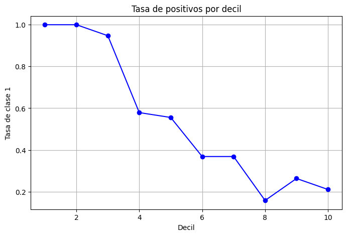
Tasa de positivos reales en test: 0.54
       Total  Positivos      Tasa      Lift  Captura_Acum
Decil
1         19         19  1.000000  1.834951      0.184466
2         19         18  0.947368  1.738375      0.359223
3         19         18  0.947368  1.738375      0.533981
4         19         11  0.578947  1.062340      0.640777
5         18         11  0.611111  1.121359      0.747573
6         19          6  0.315789  0.579458      0.805825
7         19          8  0.421053  0.772611      0.883495
8         19          6  0.315789  0.579458      0.941748
9         19          4  0.210526  0.386306      0.980583
10        19          2  0.105263  0.193153      1.000000
Cambio de umbral:#
# Crear lista de umbrales a evaluar
umbrales = np.arange(0.1, 0.91, 0.05)

# Lista para almacenar resultados
resultados = []

for umbral in umbrales:
    y_pred_umbral = (y_prob >= umbral).astype(int)
    tn, fp, fn, tp = confusion_matrix(y_test, y_pred_umbral).ravel()

    precision = precision_score(y_test, y_pred_umbral, zero_division=0)
    recall = recall_score(y_test, y_pred_umbral)
    specificity = tn / (tn + fp)
    accuracy = accuracy_score(y_test, y_pred_umbral)
    f1 = f1_score(y_test, y_pred_umbral)

    resultados.append({
        'Umbral': umbral,
        'Precision': precision,
        'Recall (Sensibilidad)': recall,
        'Especificidad': specificity,
        'Accuracy': accuracy,
        'F1-score': f1
    })

# Convertir a DataFrame
df_resultados = pd.DataFrame(resultados)

# Mostrar tabla
plt.figure(figsize=(12, 6))
sns.lineplot(data=df_resultados.set_index('Umbral'))
plt.title('Métricas por Umbral de Decisión')
plt.ylabel('Valor')
plt.gca().yaxis.set_major_formatter(mtick.PercentFormatter(1.0))
plt.grid(True)
plt.show()

df_resultados
| Umbral | Precision | Recall (Sensibilidad) | Especificidad | Accuracy | F1-score | |
|---|---|---|---|---|---|---|
| 0 | 0.10 | 0.551351 | 0.990291 | 0.034884 | 0.555556 | 0.708333 |
| 1 | 0.15 | 0.576271 | 0.990291 | 0.127907 | 0.597884 | 0.728571 |
| 2 | 0.20 | 0.611111 | 0.961165 | 0.267442 | 0.645503 | 0.747170 |
| 3 | 0.25 | 0.648649 | 0.932039 | 0.395349 | 0.687831 | 0.764940 |
| 4 | 0.30 | 0.686567 | 0.893204 | 0.511628 | 0.719577 | 0.776371 |
| 5 | 0.35 | 0.705426 | 0.883495 | 0.558140 | 0.735450 | 0.784483 |
| 6 | 0.40 | 0.722689 | 0.834951 | 0.616279 | 0.735450 | 0.774775 |
| 7 | 0.45 | 0.736364 | 0.786408 | 0.662791 | 0.730159 | 0.760563 |
| 8 | 0.50 | 0.806122 | 0.766990 | 0.779070 | 0.772487 | 0.786070 |
| 9 | 0.55 | 0.817204 | 0.737864 | 0.802326 | 0.767196 | 0.775510 |
| 10 | 0.60 | 0.835294 | 0.689320 | 0.837209 | 0.756614 | 0.755319 |
| 11 | 0.65 | 0.870130 | 0.650485 | 0.883721 | 0.756614 | 0.744444 |
| 12 | 0.70 | 0.909091 | 0.582524 | 0.930233 | 0.740741 | 0.710059 |
| 13 | 0.75 | 0.904762 | 0.553398 | 0.930233 | 0.724868 | 0.686747 |
| 14 | 0.80 | 0.964286 | 0.524272 | 0.976744 | 0.730159 | 0.679245 |
| 15 | 0.85 | 0.980392 | 0.485437 | 0.988372 | 0.714286 | 0.649351 |
| 16 | 0.90 | 0.975000 | 0.378641 | 0.988372 | 0.656085 | 0.545455 |
umbral_optimo = 0.45

y_pred_final = (y_prob >= umbral_optimo).astype(int)

cm_df_final = confusion_matrix(y_test, y_pred_final)

plt.figure(figsize=(5.2,4.2))
sns.heatmap(cm_df_final, annot=True, fmt="d", cbar=True, linewidths=.5, cmap="coolwarm")
plt.title("Matriz de confusión - Test")
plt.xlabel("Predicho"); plt.ylabel("Real")
plt.tight_layout()
plt.show()

print("\nReporte de Clasificación:")
print(classification_report(y_test, y_pred_final))

print(f"ROC AUC: {roc_auc_score(y_test, y_prob):.3f}")
Reporte de Clasificación:
              precision    recall  f1-score   support

           0       0.72      0.66      0.69        86
           1       0.74      0.79      0.76       103

    accuracy                           0.73       189
   macro avg       0.73      0.72      0.73       189
weighted avg       0.73      0.73      0.73       189

ROC AUC: 0.847
# DataFrame con probas y clase real
df_deciles = pd.DataFrame({'y_real': y_pred_final, 'y_proba': y_prob})

# Crear deciles (1 = más alto riesgo, 10 = más bajo)
df_deciles['Decil'] = pd.qcut(df_deciles['y_proba'], 10, labels=False, duplicates='drop') + 1
df_deciles['Decil'] = 11 - df_deciles['Decil']   # invertir para que el decil 1 sea el de mayor riesgo

# Calcular tasa por decil
tabla_deciles = df_deciles.groupby('Decil').agg(
    Total=('y_real','count'),
    Positivos=('y_real','sum')
)
tabla_deciles['Tasa'] = tabla_deciles['Positivos'] / tabla_deciles['Total']
tabla_deciles['Lift'] = tabla_deciles['Tasa'] / df_deciles['y_real'].mean()
tabla_deciles['Captura_Acum'] = tabla_deciles['Positivos'].cumsum() / df_deciles['y_real'].sum()

print(f"Tasa de positivos reales en test: {df_deciles['y_real'].mean():.2f}")

print(tabla_deciles)

# --- 📊 Gráfico ---
plt.figure(figsize=(8,5))
plt.plot(tabla_deciles.index, tabla_deciles['Tasa'], marker='o', linestyle='-', color='blue')
plt.title("Tasa de positivos por decil")
plt.xlabel("Decil")
plt.ylabel("Tasa de clase 1")
plt.grid(True)
plt.show()
Tasa de positivos reales en test: 0.58
       Total  Positivos      Tasa      Lift  Captura_Acum
Decil
1         19         19  1.000000  1.718182      0.172727
2         19         19  1.000000  1.718182      0.345455
3         19         19  1.000000  1.718182      0.518182
4         19         19  1.000000  1.718182      0.690909
5         18         18  1.000000  1.718182      0.854545
6         19         16  0.842105  1.446890      1.000000
7         19          0  0.000000  0.000000      1.000000
8         19          0  0.000000  0.000000      1.000000
9         19          0  0.000000  0.000000      1.000000
10        19          0  0.000000  0.000000      1.000000
Cambio de parámetros:#
# ------------------------
# Ajustar el modelo
# ------------------------
model = SVC(kernel="rbf", probability=True, C=10, gamma=0.3)
model.fit(X_train, y_train)

# ------------------------
# Predicciones
# ------------------------
y_pred_train = model.predict(X_train)
y_prob_train = model.predict_proba(X_train)[:, 1]

y_pred = model.predict(X_test)
y_prob = model.predict_proba(X_test)[:, 1]

# ------------------------
# Evaluación del modelo
# ------------------------
print("\n=== Reporte de Clasificación - train ===")
print(classification_report(y_train, y_pred_train))

print("\n=== Reporte de Clasificación - test ===")
print(classification_report(y_test, y_pred))

# DataFrame con probas y clase real
df_deciles = pd.DataFrame({'y_real': y_test, 'y_proba': y_prob})

# Crear deciles (1 = más alto riesgo, 10 = más bajo)
df_deciles['Decil'] = pd.qcut(df_deciles['y_proba'], 10, labels=False, duplicates='drop') + 1
df_deciles['Decil'] = 11 - df_deciles['Decil']   # invertir para que el decil 1 sea el de mayor riesgo

# Calcular tasa por decil
tabla_deciles = df_deciles.groupby('Decil').agg(
    Total=('y_real','count'),
    Positivos=('y_real','sum')
)
tabla_deciles['Tasa'] = tabla_deciles['Positivos'] / tabla_deciles['Total']
tabla_deciles['Lift'] = tabla_deciles['Tasa'] / df_deciles['y_real'].mean()
tabla_deciles['Captura_Acum'] = tabla_deciles['Positivos'].cumsum() / df_deciles['y_real'].sum()

# --- 📊 Gráfico ---
plt.figure(figsize=(8,5))
plt.plot(tabla_deciles.index, tabla_deciles['Tasa'], marker='o', linestyle='-', color='blue')
plt.title("Tasa de positivos por decil")
plt.xlabel("Decil")
plt.ylabel("Tasa de clase 1")
plt.grid(True)
plt.show()
=== Reporte de Clasificación - train ===
              precision    recall  f1-score   support

           0       0.75      0.94      0.83       201
           1       0.94      0.73      0.82       239

    accuracy                           0.83       440
   macro avg       0.84      0.84      0.83       440
weighted avg       0.85      0.83      0.83       440


=== Reporte de Clasificación - test ===
              precision    recall  f1-score   support

           0       0.71      0.84      0.77        86
           1       0.84      0.72      0.77       103

    accuracy                           0.77       189
   macro avg       0.78      0.78      0.77       189
weighted avg       0.78      0.77      0.77       189