GridSearchCV#
import pandas as pd
import numpy as np
import matplotlib.pyplot as plt
from sklearn.model_selection import train_test_split
from sklearn.preprocessing import StandardScaler
from keras.models import Sequential
from keras.layers import Dense
import keras
import warnings  # Para ignorar mensajes de advertencia

warnings.filterwarnings("ignore")
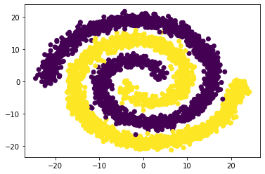
df = pd.read_csv("spiral.csv", sep=",", decimal=".")
print(df.head())
         X1        X2    y
0  13.31596  -5.47317  0.0
1  16.70656   1.26700  0.0
2   7.18348   7.29934  1.0
3  -7.94940 -14.77444  1.0
4  -5.96108 -18.68620  1.0
plt.scatter(df.iloc[:,0],df.iloc[:,1], c = df.iloc[:,2])
plt.show()
Conjunto de train y test:#
X = pd.concat([df[["X1", "X2"]]], axis=1)
print(X)
            X1        X2
0     13.31596  -5.47317
1     16.70656   1.26700
2      7.18348   7.29934
3     -7.94940 -14.77444
4     -5.96108 -18.68620
...        ...       ...
3995   4.67165  11.72679
3996  -9.34366   0.81879
3997 -13.08116 -14.54117
3998  10.66048 -17.28003
3999  12.35733  -8.63444

[4000 rows x 2 columns]
y = df["y"]
print(y)
0       0.0
1       0.0
2       1.0
3       1.0
4       1.0
       ...
3995    1.0
3996    0.0
3997    1.0
3998    1.0
3999    0.0
Name: y, Length: 4000, dtype: float64
X_train, X_test, y_train, y_test = train_test_split(X, y, test_size=0.2, random_state=0)
Escalado de variables:#
sc = StandardScaler()
sc.fit(X_train)
X_train = sc.transform(X_train)
X_test = sc.transform(X_test)
GridSearchCV pertenece a Scikit-Learn y los modelos de redes
neuronales los estamos creando en Keras; sin embargo, podemos usar
herramientas de Scikit-Learn sobre los trabajado en Keras por medio de
tf.keras.wrappers.scikit_learn que usa la API de Scikit-Learn con
modelos Keras.
Esto se pude usar tanto para clasificación como para regresión:
Optimización de neuronas y epochs:#
Construcción de la red neuronal:
def create_model(units = 1):

    model = Sequential()
    model.add(Dense(units, activation = "relu", input_shape=(X.shape[1],)))
    model.add(Dense(units, activation = "relu"))
    model.add(Dense(1, activation = "sigmoid"))
    model.compile(loss = "binary_crossentropy", optimizer = "adam", metrics = ["accuracy"])

    return model
Hiperparámetros a ajustar:
Creamos una lista de hiperparámetros y de los valores que cada uno tendrá.
param_grid = dict(units = [4, 6], epochs = [50, 100])
param_grid
{'units': [4, 6], 'epochs': [50, 100]}
Con los valores indicados en param_grid se entrenará el modelo
varias veces con todas las combinaciones posibles de los hiperparámetros
que queremos optimizar, en este caso, se entrenará el modelo con 4
neuronas en cada capa y se hará 2 veces, el primero con 50 epochs y el
segundo con 100. Luego cambiará la arquitectura a 6 neuronas por capa y
repetirá el proceso con la misma secuencia de epochs. En total realizará
4 entrenamientos.
Uso de la API de Scikit-Learn sobre Keras:
from keras.wrappers.scikit_learn import KerasClassifier
keras_reg = KerasClassifier(create_model, verbose = 1)
GridSearchCV de Scikit-Learn para optimizar hiperparámetros:
from sklearn.model_selection import GridSearchCV
El entrenamiento se realiza con cross-validation que por defecto usa
cinco subconjuntos de datos aleatorios. El argumento para cambiarlo es
cv= (por defecto es cv=5).
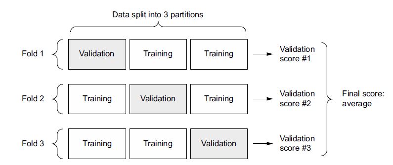
K-fold#
Tenemos en param_grid dos configuraciones para units y dos
configuraciones para epochs, para un total de cuatro combinaciones
de hiperparámetros para entrenar el modelo, pero como cv=5,
entonces, realizará 20 corridas (4 combinaciones \(\times\) 5 de
cross-validation).
grid_search = GridSearchCV(estimator=keras_reg, param_grid=param_grid)
El método .fit() es el mismo usado en Keras con el Sequential()
models. Los argumentos que más usamos son:
fit(x=None, y=None, batch_size=None, epochs=1, verbose=1, callbacks=None, validation_split=0.0, validation_data=None)
Al final de probar todas las combinaciones de hiperparámtros, automáticamente vuelve a entrenar el modelo con el mejor, pero con todos los datos.
grid_search.fit(X_train, y_train,
        validation_data = (X_test, y_test),
        verbose = 0)
20/20 [==============================] - 0s 822us/step - loss: 0.5112 - accuracy: 0.7031
20/20 [==============================] - 0s 874us/step - loss: 0.4240 - accuracy: 0.7578
20/20 [==============================] - 0s 840us/step - loss: 0.4754 - accuracy: 0.7266
20/20 [==============================] - 0s 945us/step - loss: 0.4457 - accuracy: 0.7406
20/20 [==============================] - 0s 891us/step - loss: 0.5746 - accuracy: 0.6562
20/20 [==============================] - 0s 818us/step - loss: 0.4308 - accuracy: 0.8219
20/20 [==============================] - 0s 945us/step - loss: 0.3322 - accuracy: 0.8578
20/20 [==============================] - 0s 894us/step - loss: 0.3926 - accuracy: 0.8125
20/20 [==============================] - 0s 840us/step - loss: 0.5040 - accuracy: 0.6859
20/20 [==============================] - 0s 892us/step - loss: 0.4283 - accuracy: 0.7734
20/20 [==============================] - 0s 892us/step - loss: 0.3485 - accuracy: 0.8234
20/20 [==============================] - 0s 1ms/step - loss: 0.5925 - accuracy: 0.6484
20/20 [==============================] - 0s 998us/step - loss: 0.2371 - accuracy: 0.8984
20/20 [==============================] - 0s 1ms/step - loss: 0.4748 - accuracy: 0.7094
20/20 [==============================] - 0s 945us/step - loss: 0.3069 - accuracy: 0.8687
20/20 [==============================] - 0s 840us/step - loss: 0.1897 - accuracy: 0.9500
20/20 [==============================] - 0s 855us/step - loss: 0.3159 - accuracy: 0.8516
20/20 [==============================] - 0s 822us/step - loss: 0.1218 - accuracy: 0.9828
20/20 [==============================] - 0s 883us/step - loss: 0.2726 - accuracy: 0.8781
20/20 [==============================] - 0s 1ms/step - loss: 0.2500 - accuracy: 0.8797
GridSearchCV(estimator=<keras.wrappers.scikit_learn.KerasClassifier object at 0x000002858AD34670>,
             param_grid={'epochs': [50, 100], 'units': [4, 6]})
Configuraciones de hiperparámetros:
grid_search.cv_results_["params"]
[{'epochs': 50, 'units': 4},
 {'epochs': 50, 'units': 6},
 {'epochs': 100, 'units': 4},
 {'epochs': 100, 'units': 6}]
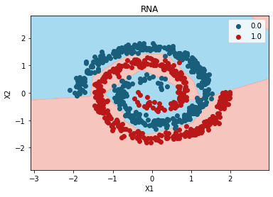
Mejor modelo:
grid_search.best_params_
{'epochs': 100, 'units': 6}
Predicción con el mejor modelo:
y_pred = grid_search.best_estimator_.predict(X_test, verbose = 0)
y_pred[0:5]
array([[0.],
       [1.],
       [0.],
       [1.],
       [0.]])
from matplotlib.colors import ListedColormap
X_Set, y_Set = X_test, y_test
X1, X2 = np.meshgrid(
np.arange(start=X_Set[:, 0].min() - 1, stop=X_Set[:, 0].max() + 1, step=0.01),
np.arange(start=X_Set[:, 1].min() - 1, stop=X_Set[:, 1].max() + 1, step=0.01),
)
plt.contourf(
X1,
X2,
grid_search.best_estimator_.predict(np.array([X1.ravel(), X2.ravel()]).T).reshape(X1.shape),
alpha=0.75,
cmap=ListedColormap(("skyblue", "#F3B3A9"))
)
plt.xlim(X1.min(), X1.max())
plt.ylim(X2.min(), X2.max())
for i, j in enumerate(np.unique(y_Set)):
plt.scatter(
X_Set[y_Set == j, 0],
X_Set[y_Set == j, 1],
c=ListedColormap(("#195E7A", "#BA1818"))(i),
label=j,
)
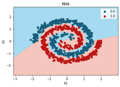
plt.title("RNA")
plt.xlabel("X1")
plt.ylabel("X2")
plt.legend()
plt.show()
10715/10715 [==============================] - 8s 766us/step
c argument looks like a single numeric RGB or RGBA sequence, which should be avoided as value-mapping will have precedence in case its length matches with x & y.  Please use the color keyword-argument or provide a 2D array with a single row if you intend to specify the same RGB or RGBA value for all points.
c argument looks like a single numeric RGB or RGBA sequence, which should be avoided as value-mapping will have precedence in case its length matches with x & y.  Please use the color keyword-argument or provide a 2D array with a single row if you intend to specify the same RGB or RGBA value for all points.
Optimización de función de activación:#
Construcción de la red neuronal:
def create_model(activation = "relu"):

    model = Sequential()
    model.add(Dense(6, activation = activation, input_shape=(X.shape[1],)))
    model.add(Dense(6, activation = activation))
    model.add(Dense(1, activation = "sigmoid"))
    model.compile(loss = "binary_crossentropy", optimizer = "adam", metrics = ["accuracy"])

    return model
Hiperparámetro a ajustar:
param_grid = dict(activation = ["relu", "sigmoid", "tanh"])
param_grid
{'activation': ['relu', 'sigmoid', 'tanh']}
Uso de la API de Scikit-Learn sobre Keras:
keras_reg = KerasClassifier(create_model, verbose = 1)
GridSearchCV de Scikit-Learn para optimizar hiperparámetros:
grid_search = GridSearchCV(estimator=keras_reg, param_grid=param_grid)
import time

StartTime = time.time()

grid_search.fit(X_train, y_train,
        validation_data = (X_test, y_test),
        verbose = 0,
        epochs = 150)

EndTime = time.time()
print("---------> Tiempo en procesar: ", round((EndTime - StartTime) / 60), "Minutos")
20/20 [==============================] - 0s 2ms/step - loss: 0.1207 - accuracy: 0.9594
20/20 [==============================] - 0s 939us/step - loss: 0.1206 - accuracy: 0.9594
20/20 [==============================] - 0s 820us/step - loss: 0.1430 - accuracy: 0.9406
20/20 [==============================] - 0s 820us/step - loss: 0.1444 - accuracy: 0.9281
20/20 [==============================] - 0s 842us/step - loss: 0.1493 - accuracy: 0.9609
20/20 [==============================] - 0s 820us/step - loss: 0.6313 - accuracy: 0.6297
20/20 [==============================] - 0s 894us/step - loss: 0.6163 - accuracy: 0.6797
20/20 [==============================] - 0s 866us/step - loss: 0.6186 - accuracy: 0.6609
20/20 [==============================] - 0s 820us/step - loss: 0.6210 - accuracy: 0.6750
20/20 [==============================] - 0s 1ms/step - loss: 0.6282 - accuracy: 0.6438
20/20 [==============================] - 0s 998us/step - loss: 0.4419 - accuracy: 0.8031
20/20 [==============================] - 0s 927us/step - loss: 0.5045 - accuracy: 0.7422
20/20 [==============================] - 0s 2ms/step - loss: 0.4123 - accuracy: 0.8125
20/20 [==============================] - 0s 821us/step - loss: 0.4798 - accuracy: 0.7875
20/20 [==============================] - 0s 822us/step - loss: 0.4127 - accuracy: 0.8344
---------> Tiempo en procesar:  4 Minutos
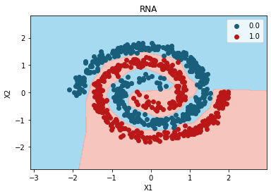
Mejor modelo:
grid_search.best_params_
{'activation': 'relu'}
Predicción con el mejor modelo:
y_pred = grid_search.best_estimator_.predict(X_test, verbose = 0)
y_pred[0:5]
array([[0.],
       [1.],
       [0.],
       [1.],
       [0.]])
from matplotlib.colors import ListedColormap

X_Set, y_Set = X_test, y_test
X1, X2 = np.meshgrid(
    np.arange(start=X_Set[:, 0].min() - 1, stop=X_Set[:, 0].max() + 1, step=0.01),
    np.arange(start=X_Set[:, 1].min() - 1, stop=X_Set[:, 1].max() + 1, step=0.01),
)
plt.contourf(
    X1,
    X2,
    grid_search.best_estimator_.predict(np.array([X1.ravel(), X2.ravel()]).T).reshape(X1.shape),
    alpha=0.75,
    cmap=ListedColormap(("skyblue", "#F3B3A9")), verbose = 0
)
plt.xlim(X1.min(), X1.max())
plt.ylim(X2.min(), X2.max())
for i, j in enumerate(np.unique(y_Set)):
    plt.scatter(
        X_Set[y_Set == j, 0],
        X_Set[y_Set == j, 1],
        c=ListedColormap(("#195E7A", "#BA1818"))(i),
        label=j,
    )
plt.title("RNA")
plt.xlabel("X1")
plt.ylabel("X2")
plt.legend()
plt.show()
10715/10715 [==============================] - 7s 683us/step
c argument looks like a single numeric RGB or RGBA sequence, which should be avoided as value-mapping will have precedence in case its length matches with x & y.  Please use the color keyword-argument or provide a 2D array with a single row if you intend to specify the same RGB or RGBA value for all points.
c argument looks like a single numeric RGB or RGBA sequence, which should be avoided as value-mapping will have precedence in case its length matches with x & y.  Please use the color keyword-argument or provide a 2D array with a single row if you intend to specify the same RGB or RGBA value for all points.
Optimización de la cantidad de capas ocultas:#
Construcción de la red neuronal:
def create_model(n_hidden = 2):

    model = Sequential()

    # Dimensión de las entradas para la primera capa:
    model.add(keras.layers.InputLayer(input_shape=(X.shape[1],)))

    # Loop para las capas ocultas:
    for layer in range(n_hidden):
        model.add(Dense(6, activation="relu"))

    model.add(Dense(1, activation = "sigmoid"))
    model.compile(loss = "binary_crossentropy", optimizer = "adam", metrics = ["accuracy"])

    return model
Hiperparámetro a ajustar:
param_grid = dict(n_hidden = [2, 3, 4])
param_grid
{'n_hidden': [2, 3, 4]}
Uso de la API de Scikit-Learn sobre Keras:
keras_reg = KerasClassifier(create_model, verbose = 1)
GridSearchCV de Scikit-Learn para optimizar hiperparámetros:
grid_search = GridSearchCV(estimator=keras_reg, param_grid=param_grid)
grid_search.fit(X_train, y_train,
        validation_data = (X_test, y_test),
        verbose = 0,
        epochs = 150)
20/20 [==============================] - 0s 805us/step - loss: 0.2623 - accuracy: 0.8859
20/20 [==============================] - 0s 1ms/step - loss: 0.0531 - accuracy: 0.9844
20/20 [==============================] - 0s 1ms/step - loss: 0.2051 - accuracy: 0.8906
20/20 [==============================] - 0s 789us/step - loss: 0.2500 - accuracy: 0.8797
20/20 [==============================] - 0s 953us/step - loss: 0.1040 - accuracy: 0.9609
20/20 [==============================] - 0s 820us/step - loss: 0.0424 - accuracy: 0.9891
20/20 [==============================] - 0s 822us/step - loss: 0.0308 - accuracy: 0.9922
20/20 [==============================] - 0s 822us/step - loss: 0.0297 - accuracy: 0.9922
20/20 [==============================] - 0s 822us/step - loss: 0.0179 - accuracy: 0.9969
20/20 [==============================] - 0s 882us/step - loss: 0.0340 - accuracy: 0.9859
20/20 [==============================] - 0s 821us/step - loss: 0.0225 - accuracy: 0.9906
20/20 [==============================] - 0s 822us/step - loss: 0.0271 - accuracy: 0.9922
20/20 [==============================] - 0s 822us/step - loss: 0.0432 - accuracy: 0.9859
20/20 [==============================] - 0s 877us/step - loss: 0.0498 - accuracy: 0.9875
20/20 [==============================] - 0s 822us/step - loss: 0.0677 - accuracy: 0.9625
GridSearchCV(estimator=<keras.wrappers.scikit_learn.KerasClassifier object at 0x00000285969B6D30>,
             param_grid={'n_hidden': [2, 3, 4]})
Mejor modelo:
grid_search.best_params_
{'n_hidden': 3}
Predicción con el mejor modelo:
y_pred = grid_search.best_estimator_.predict(X_test, verbose = 0)
y_pred[0:5]
array([[0.],
       [1.],
       [0.],
       [1.],
       [0.]])
from matplotlib.colors import ListedColormap
X_Set, y_Set = X_test, y_test
X1, X2 = np.meshgrid(
np.arange(start=X_Set[:, 0].min() - 1, stop=X_Set[:, 0].max() + 1, step=0.01),
np.arange(start=X_Set[:, 1].min() - 1, stop=X_Set[:, 1].max() + 1, step=0.01),
)
plt.contourf(
X1,
X2,
grid_search.best_estimator_.predict(np.array([X1.ravel(), X2.ravel()]).T).reshape(X1.shape),
alpha=0.75,
cmap=ListedColormap(("skyblue", "#F3B3A9")), verbose = 0
)
plt.xlim(X1.min(), X1.max())
plt.ylim(X2.min(), X2.max())
for i, j in enumerate(np.unique(y_Set)):
plt.scatter(
X_Set[y_Set == j, 0],
X_Set[y_Set == j, 1],
c=ListedColormap(("#195E7A", "#BA1818"))(i),
label=j,
)
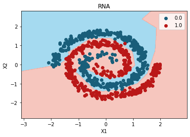
plt.title("RNA")
plt.xlabel("X1")
plt.ylabel("X2")
plt.legend()
plt.show()
10715/10715 [==============================] - 7s 681us/step
c argument looks like a single numeric RGB or RGBA sequence, which should be avoided as value-mapping will have precedence in case its length matches with x & y.  Please use the color keyword-argument or provide a 2D array with a single row if you intend to specify the same RGB or RGBA value for all points.
c argument looks like a single numeric RGB or RGBA sequence, which should be avoided as value-mapping will have precedence in case its length matches with x & y.  Please use the color keyword-argument or provide a 2D array with a single row if you intend to specify the same RGB or RGBA value for all points.
Optimización de neuronas, capas ocultas, función de activación, optimizadores, batch y epochs:#
Construcción de la red neuronal:
def create_model(units = 1, n_hidden = 2, activation = "relu", optimizer = "adam"):

    model = Sequential()

    # Dimensión de las entradas para la primera capa:
    model.add(keras.layers.InputLayer(input_shape=(X.shape[1],)))

    # Loop para las capas ocultas:
    for layer in range(n_hidden):
        model.add(Dense(units, activation=activation))

    model.add(Dense(1, activation = "sigmoid"))
    model.compile(loss = "binary_crossentropy", optimizer = optimizer, metrics = ["accuracy"])

    return model
Hiperparámetros a ajustar:
Algunos hiperparámetros están dentro de la función creada llamada
create_model(), los demás hiperparámtros que están por fuera de esta
función y que pertenecen al método .fit() deben tener el mismo
nombre que los argumentos, por ejemplo, los hiperparámetros
batch_size y epochs.
param_grid = dict(units = [4, 6],
                  n_hidden = [2, 3],
                  activation = ["relu", "tanh", "sigmoid"],
                  optimizer = ["adam", "rmsprop"],
                  batch_size = [10, 50],
                  epochs = [50, 100])
param_grid
{'units': [4, 6],
 'n_hidden': [2, 3],
 'activation': ['relu', 'tanh', 'sigmoid'],
 'optimizer': ['adam', 'rmsprop'],
 'batch_size': [10, 50],
 'epochs': [50, 100]}
Uso de la API de Scikit-Learn sobre Keras:
keras_reg = KerasClassifier(create_model, verbose = 0)
GridSearchCV de Scikit-Learn para optimizar hiperparámetros:
grid_search = GridSearchCV(estimator=keras_reg, param_grid=param_grid, n_jobs=-1)
StartTime = time.time()

grid_search.fit(X_train, y_train,
        validation_data = (X_test, y_test),
        verbose = 0)

EndTime = time.time()
print("---------> Tiempo en procesar: ", round((EndTime - StartTime) / 60), "Minutos")
---------> Tiempo en procesar: 37 Minutos
Configuraciones de hiperparámetros:
grid_search.cv_results_["params"]
[{'activation': 'relu',
  'batch_size': 10,
  'epochs': 50,
  'n_hidden': 2,
  'optimizer': 'adam',
  'units': 4},
 {'activation': 'relu',
  'batch_size': 10,
  'epochs': 50,
  'n_hidden': 2,
  'optimizer': 'adam',
  'units': 6},
 {'activation': 'relu',
  'batch_size': 10,
  'epochs': 50,
  'n_hidden': 2,
  'optimizer': 'rmsprop',
  'units': 4},
 {'activation': 'relu',
  'batch_size': 10,
  'epochs': 50,
  'n_hidden': 2,
  'optimizer': 'rmsprop',
  'units': 6},
 {'activation': 'relu',
  'batch_size': 10,
  'epochs': 50,
  'n_hidden': 3,
  'optimizer': 'adam',
  'units': 4},
 {'activation': 'relu',
  'batch_size': 10,
  'epochs': 50,
  'n_hidden': 3,
  'optimizer': 'adam',
  'units': 6},
 {'activation': 'relu',
  'batch_size': 10,
  'epochs': 50,
  'n_hidden': 3,
  'optimizer': 'rmsprop',
  'units': 4},
 {'activation': 'relu',
  'batch_size': 10,
  'epochs': 50,
  'n_hidden': 3,
  'optimizer': 'rmsprop',
  'units': 6},
 {'activation': 'relu',
  'batch_size': 10,
  'epochs': 100,
  'n_hidden': 2,
  'optimizer': 'adam',
  'units': 4},
 {'activation': 'relu',
  'batch_size': 10,
  'epochs': 100,
  'n_hidden': 2,
  'optimizer': 'adam',
  'units': 6},
 {'activation': 'relu',
  'batch_size': 10,
  'epochs': 100,
  'n_hidden': 2,
  'optimizer': 'rmsprop',
  'units': 4},
 {'activation': 'relu',
  'batch_size': 10,
  'epochs': 100,
  'n_hidden': 2,
  'optimizer': 'rmsprop',
  'units': 6},
 {'activation': 'relu',
  'batch_size': 10,
  'epochs': 100,
  'n_hidden': 3,
  'optimizer': 'adam',
  'units': 4},
 {'activation': 'relu',
  'batch_size': 10,
  'epochs': 100,
  'n_hidden': 3,
  'optimizer': 'adam',
  'units': 6},
 {'activation': 'relu',
  'batch_size': 10,
  'epochs': 100,
  'n_hidden': 3,
  'optimizer': 'rmsprop',
  'units': 4},
 {'activation': 'relu',
  'batch_size': 10,
  'epochs': 100,
  'n_hidden': 3,
  'optimizer': 'rmsprop',
  'units': 6},
 {'activation': 'relu',
  'batch_size': 50,
  'epochs': 50,
  'n_hidden': 2,
  'optimizer': 'adam',
  'units': 4},
 {'activation': 'relu',
  'batch_size': 50,
  'epochs': 50,
  'n_hidden': 2,
  'optimizer': 'adam',
  'units': 6},
 {'activation': 'relu',
  'batch_size': 50,
  'epochs': 50,
  'n_hidden': 2,
  'optimizer': 'rmsprop',
  'units': 4},
 {'activation': 'relu',
  'batch_size': 50,
  'epochs': 50,
  'n_hidden': 2,
  'optimizer': 'rmsprop',
  'units': 6},
 {'activation': 'relu',
  'batch_size': 50,
  'epochs': 50,
  'n_hidden': 3,
  'optimizer': 'adam',
  'units': 4},
 {'activation': 'relu',
  'batch_size': 50,
  'epochs': 50,
  'n_hidden': 3,
  'optimizer': 'adam',
  'units': 6},
 {'activation': 'relu',
  'batch_size': 50,
  'epochs': 50,
  'n_hidden': 3,
  'optimizer': 'rmsprop',
  'units': 4},
 {'activation': 'relu',
  'batch_size': 50,
  'epochs': 50,
  'n_hidden': 3,
  'optimizer': 'rmsprop',
  'units': 6},
 {'activation': 'relu',
  'batch_size': 50,
  'epochs': 100,
  'n_hidden': 2,
  'optimizer': 'adam',
  'units': 4},
 {'activation': 'relu',
  'batch_size': 50,
  'epochs': 100,
  'n_hidden': 2,
  'optimizer': 'adam',
  'units': 6},
 {'activation': 'relu',
  'batch_size': 50,
  'epochs': 100,
  'n_hidden': 2,
  'optimizer': 'rmsprop',
  'units': 4},
 {'activation': 'relu',
  'batch_size': 50,
  'epochs': 100,
  'n_hidden': 2,
  'optimizer': 'rmsprop',
  'units': 6},
 {'activation': 'relu',
  'batch_size': 50,
  'epochs': 100,
  'n_hidden': 3,
  'optimizer': 'adam',
  'units': 4},
 {'activation': 'relu',
  'batch_size': 50,
  'epochs': 100,
  'n_hidden': 3,
  'optimizer': 'adam',
  'units': 6},
 {'activation': 'relu',
  'batch_size': 50,
  'epochs': 100,
  'n_hidden': 3,
  'optimizer': 'rmsprop',
  'units': 4},
 {'activation': 'relu',
  'batch_size': 50,
  'epochs': 100,
  'n_hidden': 3,
  'optimizer': 'rmsprop',
  'units': 6},
 {'activation': 'tanh',
  'batch_size': 10,
  'epochs': 50,
  'n_hidden': 2,
  'optimizer': 'adam',
  'units': 4},
 {'activation': 'tanh',
  'batch_size': 10,
  'epochs': 50,
  'n_hidden': 2,
  'optimizer': 'adam',
  'units': 6},
 {'activation': 'tanh',
  'batch_size': 10,
  'epochs': 50,
  'n_hidden': 2,
  'optimizer': 'rmsprop',
  'units': 4},
 {'activation': 'tanh',
  'batch_size': 10,
  'epochs': 50,
  'n_hidden': 2,
  'optimizer': 'rmsprop',
  'units': 6},
 {'activation': 'tanh',
  'batch_size': 10,
  'epochs': 50,
  'n_hidden': 3,
  'optimizer': 'adam',
  'units': 4},
 {'activation': 'tanh',
  'batch_size': 10,
  'epochs': 50,
  'n_hidden': 3,
  'optimizer': 'adam',
  'units': 6},
 {'activation': 'tanh',
  'batch_size': 10,
  'epochs': 50,
  'n_hidden': 3,
  'optimizer': 'rmsprop',
  'units': 4},
 {'activation': 'tanh',
  'batch_size': 10,
  'epochs': 50,
  'n_hidden': 3,
  'optimizer': 'rmsprop',
  'units': 6},
 {'activation': 'tanh',
  'batch_size': 10,
  'epochs': 100,
  'n_hidden': 2,
  'optimizer': 'adam',
  'units': 4},
 {'activation': 'tanh',
  'batch_size': 10,
  'epochs': 100,
  'n_hidden': 2,
  'optimizer': 'adam',
  'units': 6},
 {'activation': 'tanh',
  'batch_size': 10,
  'epochs': 100,
  'n_hidden': 2,
  'optimizer': 'rmsprop',
  'units': 4},
 {'activation': 'tanh',
  'batch_size': 10,
  'epochs': 100,
  'n_hidden': 2,
  'optimizer': 'rmsprop',
  'units': 6},
 {'activation': 'tanh',
  'batch_size': 10,
  'epochs': 100,
  'n_hidden': 3,
  'optimizer': 'adam',
  'units': 4},
 {'activation': 'tanh',
  'batch_size': 10,
  'epochs': 100,
  'n_hidden': 3,
  'optimizer': 'adam',
  'units': 6},
 {'activation': 'tanh',
  'batch_size': 10,
  'epochs': 100,
  'n_hidden': 3,
  'optimizer': 'rmsprop',
  'units': 4},
 {'activation': 'tanh',
  'batch_size': 10,
  'epochs': 100,
  'n_hidden': 3,
  'optimizer': 'rmsprop',
  'units': 6},
 {'activation': 'tanh',
  'batch_size': 50,
  'epochs': 50,
  'n_hidden': 2,
  'optimizer': 'adam',
  'units': 4},
 {'activation': 'tanh',
  'batch_size': 50,
  'epochs': 50,
  'n_hidden': 2,
  'optimizer': 'adam',
  'units': 6},
 {'activation': 'tanh',
  'batch_size': 50,
  'epochs': 50,
  'n_hidden': 2,
  'optimizer': 'rmsprop',
  'units': 4},
 {'activation': 'tanh',
  'batch_size': 50,
  'epochs': 50,
  'n_hidden': 2,
  'optimizer': 'rmsprop',
  'units': 6},
 {'activation': 'tanh',
  'batch_size': 50,
  'epochs': 50,
  'n_hidden': 3,
  'optimizer': 'adam',
  'units': 4},
 {'activation': 'tanh',
  'batch_size': 50,
  'epochs': 50,
  'n_hidden': 3,
  'optimizer': 'adam',
  'units': 6},
 {'activation': 'tanh',
  'batch_size': 50,
  'epochs': 50,
  'n_hidden': 3,
  'optimizer': 'rmsprop',
  'units': 4},
 {'activation': 'tanh',
  'batch_size': 50,
  'epochs': 50,
  'n_hidden': 3,
  'optimizer': 'rmsprop',
  'units': 6},
 {'activation': 'tanh',
  'batch_size': 50,
  'epochs': 100,
  'n_hidden': 2,
  'optimizer': 'adam',
  'units': 4},
 {'activation': 'tanh',
  'batch_size': 50,
  'epochs': 100,
  'n_hidden': 2,
  'optimizer': 'adam',
  'units': 6},
 {'activation': 'tanh',
  'batch_size': 50,
  'epochs': 100,
  'n_hidden': 2,
  'optimizer': 'rmsprop',
  'units': 4},
 {'activation': 'tanh',
  'batch_size': 50,
  'epochs': 100,
  'n_hidden': 2,
  'optimizer': 'rmsprop',
  'units': 6},
 {'activation': 'tanh',
  'batch_size': 50,
  'epochs': 100,
  'n_hidden': 3,
  'optimizer': 'adam',
  'units': 4},
 {'activation': 'tanh',
  'batch_size': 50,
  'epochs': 100,
  'n_hidden': 3,
  'optimizer': 'adam',
  'units': 6},
 {'activation': 'tanh',
  'batch_size': 50,
  'epochs': 100,
  'n_hidden': 3,
  'optimizer': 'rmsprop',
  'units': 4},
 {'activation': 'tanh',
  'batch_size': 50,
  'epochs': 100,
  'n_hidden': 3,
  'optimizer': 'rmsprop',
  'units': 6},
 {'activation': 'sigmoid',
  'batch_size': 10,
  'epochs': 50,
  'n_hidden': 2,
  'optimizer': 'adam',
  'units': 4},
 {'activation': 'sigmoid',
  'batch_size': 10,
  'epochs': 50,
  'n_hidden': 2,
  'optimizer': 'adam',
  'units': 6},
 {'activation': 'sigmoid',
  'batch_size': 10,
  'epochs': 50,
  'n_hidden': 2,
  'optimizer': 'rmsprop',
  'units': 4},
 {'activation': 'sigmoid',
  'batch_size': 10,
  'epochs': 50,
  'n_hidden': 2,
  'optimizer': 'rmsprop',
  'units': 6},
 {'activation': 'sigmoid',
  'batch_size': 10,
  'epochs': 50,
  'n_hidden': 3,
  'optimizer': 'adam',
  'units': 4},
 {'activation': 'sigmoid',
  'batch_size': 10,
  'epochs': 50,
  'n_hidden': 3,
  'optimizer': 'adam',
  'units': 6},
 {'activation': 'sigmoid',
  'batch_size': 10,
  'epochs': 50,
  'n_hidden': 3,
  'optimizer': 'rmsprop',
  'units': 4},
 {'activation': 'sigmoid',
  'batch_size': 10,
  'epochs': 50,
  'n_hidden': 3,
  'optimizer': 'rmsprop',
  'units': 6},
 {'activation': 'sigmoid',
  'batch_size': 10,
  'epochs': 100,
  'n_hidden': 2,
  'optimizer': 'adam',
  'units': 4},
 {'activation': 'sigmoid',
  'batch_size': 10,
  'epochs': 100,
  'n_hidden': 2,
  'optimizer': 'adam',
  'units': 6},
 {'activation': 'sigmoid',
  'batch_size': 10,
  'epochs': 100,
  'n_hidden': 2,
  'optimizer': 'rmsprop',
  'units': 4},
 {'activation': 'sigmoid',
  'batch_size': 10,
  'epochs': 100,
  'n_hidden': 2,
  'optimizer': 'rmsprop',
  'units': 6},
 {'activation': 'sigmoid',
  'batch_size': 10,
  'epochs': 100,
  'n_hidden': 3,
  'optimizer': 'adam',
  'units': 4},
 {'activation': 'sigmoid',
  'batch_size': 10,
  'epochs': 100,
  'n_hidden': 3,
  'optimizer': 'adam',
  'units': 6},
 {'activation': 'sigmoid',
  'batch_size': 10,
  'epochs': 100,
  'n_hidden': 3,
  'optimizer': 'rmsprop',
  'units': 4},
 {'activation': 'sigmoid',
  'batch_size': 10,
  'epochs': 100,
  'n_hidden': 3,
  'optimizer': 'rmsprop',
  'units': 6},
 {'activation': 'sigmoid',
  'batch_size': 50,
  'epochs': 50,
  'n_hidden': 2,
  'optimizer': 'adam',
  'units': 4},
 {'activation': 'sigmoid',
  'batch_size': 50,
  'epochs': 50,
  'n_hidden': 2,
  'optimizer': 'adam',
  'units': 6},
 {'activation': 'sigmoid',
  'batch_size': 50,
  'epochs': 50,
  'n_hidden': 2,
  'optimizer': 'rmsprop',
  'units': 4},
 {'activation': 'sigmoid',
  'batch_size': 50,
  'epochs': 50,
  'n_hidden': 2,
  'optimizer': 'rmsprop',
  'units': 6},
 {'activation': 'sigmoid',
  'batch_size': 50,
  'epochs': 50,
  'n_hidden': 3,
  'optimizer': 'adam',
  'units': 4},
 {'activation': 'sigmoid',
  'batch_size': 50,
  'epochs': 50,
  'n_hidden': 3,
  'optimizer': 'adam',
  'units': 6},
 {'activation': 'sigmoid',
  'batch_size': 50,
  'epochs': 50,
  'n_hidden': 3,
  'optimizer': 'rmsprop',
  'units': 4},
 {'activation': 'sigmoid',
  'batch_size': 50,
  'epochs': 50,
  'n_hidden': 3,
  'optimizer': 'rmsprop',
  'units': 6},
 {'activation': 'sigmoid',
  'batch_size': 50,
  'epochs': 100,
  'n_hidden': 2,
  'optimizer': 'adam',
  'units': 4},
 {'activation': 'sigmoid',
  'batch_size': 50,
  'epochs': 100,
  'n_hidden': 2,
  'optimizer': 'adam',
  'units': 6},
 {'activation': 'sigmoid',
  'batch_size': 50,
  'epochs': 100,
  'n_hidden': 2,
  'optimizer': 'rmsprop',
  'units': 4},
 {'activation': 'sigmoid',
  'batch_size': 50,
  'epochs': 100,
  'n_hidden': 2,
  'optimizer': 'rmsprop',
  'units': 6},
 {'activation': 'sigmoid',
  'batch_size': 50,
  'epochs': 100,
  'n_hidden': 3,
  'optimizer': 'adam',
  'units': 4},
 {'activation': 'sigmoid',
  'batch_size': 50,
  'epochs': 100,
  'n_hidden': 3,
  'optimizer': 'adam',
  'units': 6},
 {'activation': 'sigmoid',
  'batch_size': 50,
  'epochs': 100,
  'n_hidden': 3,
  'optimizer': 'rmsprop',
  'units': 4},
 {'activation': 'sigmoid',
  'batch_size': 50,
  'epochs': 100,
  'n_hidden': 3,
  'optimizer': 'rmsprop',
  'units': 6}]
Mejor modelo:
grid_search.best_params_
{'activation': 'relu',
 'batch_size': 10,
 'epochs': 100,
 'n_hidden': 3,
 'optimizer': 'adam',
 'units': 6}
Predicción con el mejor modelo:
y_pred = grid_search.best_estimator_.predict(X_test, verbose = 0)
y_pred[0:5]
array([[0.],
       [1.],
       [0.],
       [1.],
       [0.]])
from matplotlib.colors import ListedColormap

X_Set, y_Set = X_test, y_test
X1, X2 = np.meshgrid(
    np.arange(start=X_Set[:, 0].min() - 1, stop=X_Set[:, 0].max() + 1, step=0.01),
    np.arange(start=X_Set[:, 1].min() - 1, stop=X_Set[:, 1].max() + 1, step=0.01),
)
plt.contourf(
    X1,
    X2,
    grid_search.best_estimator_.predict(np.array([X1.ravel(), X2.ravel()]).T).reshape(X1.shape),
    alpha=0.75,
    cmap=ListedColormap(("skyblue", "#F3B3A9")), verbose = 0
)
plt.xlim(X1.min(), X1.max())
plt.ylim(X2.min(), X2.max())
for i, j in enumerate(np.unique(y_Set)):
    plt.scatter(
        X_Set[y_Set == j, 0],
        X_Set[y_Set == j, 1],
        c=ListedColormap(("#195E7A", "#BA1818"))(i),
        label=j,
    )
plt.title("RNA")
plt.xlabel("X1")
plt.ylabel("X2")
plt.legend()
plt.show()
10715/10715 [==============================] - 7s 658us/step
c argument looks like a single numeric RGB or RGBA sequence, which should be avoided as value-mapping will have precedence in case its length matches with x & y.  Please use the color keyword-argument or provide a 2D array with a single row if you intend to specify the same RGB or RGBA value for all points.
c argument looks like a single numeric RGB or RGBA sequence, which should be avoided as value-mapping will have precedence in case its length matches with x & y.  Please use the color keyword-argument or provide a 2D array with a single row if you intend to specify the same RGB or RGBA value for all points.