Ejemplo Regresión Logística

Datos con separación lineal:

# Ejemplo didáctico: primero los datos, luego la clasificación con Regresión Logística
# -----------------------------------------------------------------------------------
# 1) Genera datos artificiales linealmente separables (2 variables)
# 2) Grafica los datos (sin modelo)
# 3) Ajusta Regresión Logística
# 4) Grafica la clasificación del modelo (regiones)
# -----------------------------------------------------------------------------------

import numpy as np
import matplotlib.pyplot as plt
from matplotlib import lines as mlines
from sklearn.datasets import make_classification
from sklearn.linear_model import LogisticRegression
from sklearn.metrics import accuracy_score

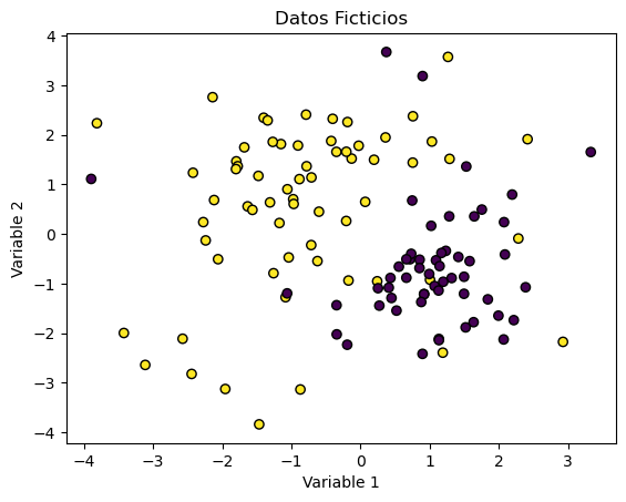
# 1) Datos ficticios con separación lineal clara
X, y = make_classification(
    n_samples=200,
    n_features=2,        # dos variables para graficar en 2D
    n_informative=2,     # ambas variables aportan información
    n_redundant=0,
    n_clusters_per_class=1,
    class_sep=2.0,       # separación clara entre clases
    random_state=42
)

# 2) Gráfica SOLO de los datos
plt.figure(figsize=(7, 6))
plt.scatter(X[:, 0], X[:, 1], c=y, s=60, edgecolor='k')
plt.title("Datos originales (2 variables)")
plt.xlabel("Variable 1")
plt.ylabel("Variable 2")
plt.grid(True, alpha=0.2)
plt.tight_layout()
plt.show()

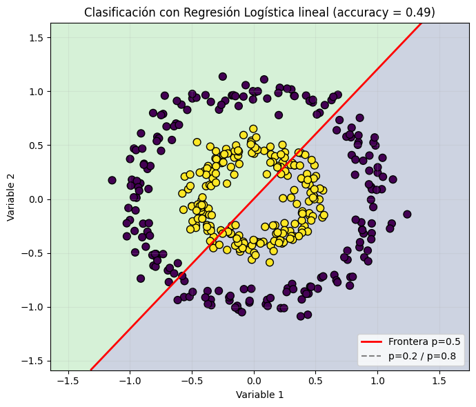
# 3) Ajustar Regresión Logística
clf = LogisticRegression()
clf.fit(X, y)
acc = accuracy_score(y, clf.predict(X))

# 4) Malla para pintar la región de decisión
x_min, x_max = X[:, 0].min() - 1, X[:, 0].max() + 1
y_min, y_max = X[:, 1].min() - 1, X[:, 1].max() + 1
xx, yy = np.meshgrid(
    np.linspace(x_min, x_max, 300),
    np.linspace(y_min, y_max, 300)
)

# Probabilidad de clase 1 en cada punto de la malla
probs = clf.predict_proba(np.c_[xx.ravel(), yy.ravel()])[:, 1].reshape(xx.shape)
Z = (probs >= 0.5).astype(int)  # clasificación final para colorear regiones

# 5) Gráfica de la CLASIFICACIÓN del modelo
plt.figure(figsize=(7, 6))

# Fondo: regiones de decisión (0/1)
plt.contourf(xx, yy, Z, alpha=0.25, levels=[-0.5, 0.5, 1.5])

# Frontera p=0.5 (como contorno)
cont_p05 = plt.contour(xx, yy, probs, levels=[0.5], colors='red', linewidths=2)

# Curvas extra de probabilidad (opcionales: 0.2 y 0.8)
plt.contour(xx, yy, probs, levels=[0.2, 0.8], colors='gray', linestyles='--', linewidths=1)

# Puntos originales
plt.scatter(X[:, 0], X[:, 1], c=y, s=60, edgecolor='k')

plt.title(f"Clasificación con Regresión Logística (accuracy = {acc:.3f})")
plt.xlabel("Variable 1")
plt.ylabel("Variable 2")
plt.grid(True, alpha=0.2)

# Leyenda robusta (compatible con distintas versiones de matplotlib)
boundary_handle = mlines.Line2D([], [], color='red', linewidth=2, label='Frontera p=0.5')
iso_handle = mlines.Line2D([], [], color='gray', linestyle='--', label='p=0.2 / p=0.8')
plt.legend(handles=[boundary_handle, iso_handle], loc='lower right')

plt.tight_layout()
plt.show()

Datos con separación no lineal:

from sklearn.datasets import make_circles

# 1) Datos no linealmente separables
X, y = make_circles(n_samples=400, factor=0.45, noise=0.08, random_state=42)

# 2) Gráfica SOLO de los datos
plt.figure(figsize=(7, 6))
plt.scatter(X[:, 0], X[:, 1], c=y, s=60, edgecolor='k')
plt.title("Datos originales (NO linealmente separables)")
plt.xlabel("Variable 1")
plt.ylabel("Variable 2")
plt.grid(True, alpha=0.2)
plt.tight_layout()
plt.show()

# 3) Ajustar Regresión Logística
clf = LogisticRegression()
clf.fit(X, y)

# Accuracy sobre TODOS los datos
acc = accuracy_score(y, clf.predict(X))
print(f"Accuracy (todo el dataset): {acc:.3f}")

# 4) Malla para pintar la región de decisión
x_min, x_max = X[:, 0].min() - 0.5, X[:, 0].max() + 0.5
y_min, y_max = X[:, 1].min() - 0.5, X[:, 1].max() + 0.5
xx, yy = np.meshgrid(
    np.linspace(x_min, x_max, 350),
    np.linspace(y_min, y_max, 350)
)

probs = clf.predict_proba(np.c_[xx.ravel(), yy.ravel()])[:, 1].reshape(xx.shape)
Z = (probs >= 0.5).astype(int)

# 5) Gráfica de la CLASIFICACIÓN del modelo
plt.figure(figsize=(7, 6))

# Fondo: regiones de decisión
plt.contourf(xx, yy, Z, alpha=0.25, levels=[-0.5, 0.5, 1.5])

# Frontera p=0.5
plt.contour(xx, yy, probs, levels=[0.5], colors='red', linewidths=2)

# Líneas opcionales de probabilidad p=0.2 y p=0.8
plt.contour(xx, yy, probs, levels=[0.2, 0.8], colors='gray', linestyles='--', linewidths=1)

# Puntos originales
plt.scatter(X[:, 0], X[:, 1], c=y, s=60, edgecolor='k')

plt.title(f"Clasificación con Regresión Logística lineal (accuracy = {acc:.2f})")
plt.xlabel("Variable 1")
plt.ylabel("Variable 2")
plt.grid(True, alpha=0.2)

# Leyenda manual
boundary_handle = mlines.Line2D([], [], color='red', linewidth=2, label='Frontera p=0.5')
iso_handle = mlines.Line2D([], [], color='gray', linestyle='--', label='p=0.2 / p=0.8')
plt.legend(handles=[boundary_handle, iso_handle], loc='lower right')

plt.tight_layout()
plt.show()

Accuracy (todo el dataset): 0.495