SVM - Regresión - código
Importar librerías:
import pandas as pd
import numpy as np
import matplotlib.pyplot as plt
Importar datos:
df = pd.read_csv("regresion.csv", sep=";", decimal=",")
print(df.head())
      X     y
0   9.0  44.7
1  10.1  78.0
2  11.6  83.0
3   9.1  80.0
4   9.7  77.0
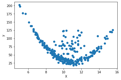
Visualización de los datos:
plt.scatter(df["X"], df["y"])
plt.xlabel("X")
plt.ylabel("y")
Text(0, 0.5, 'y')
Ajuste del modelo:
X = df[["X"]]
print(X.head())
      X
0   9.0
1  10.1
2  11.6
3   9.1
4   9.7
y = df["y"]
print(y.head())
0    44.7
1    78.0
2    83.0
3    80.0
4    77.0
Name: y, dtype: float64
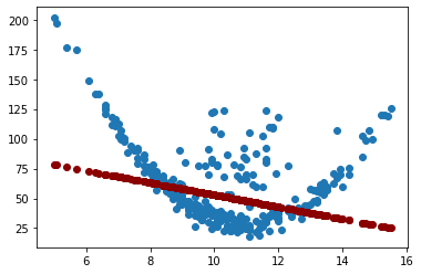
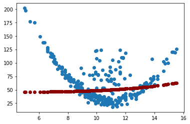
Regresión lineal:
from sklearn.svm import SVR
svm_reg = SVR(kernel="linear")
svm_reg.fit(X, y)
y_pred = svm_reg.predict(X)
Evaluación del desempeño:
from sklearn.metrics import r2_score, mean_squared_error
r2_score(y, y_pred)
0.025315275959217898
mean_squared_error(y, y_pred)
1030.9657295221316
plt.scatter(X, y)
plt.scatter(X.values, y_pred, color="darkred")
<matplotlib.collections.PathCollection at 0x1cd413c8820>
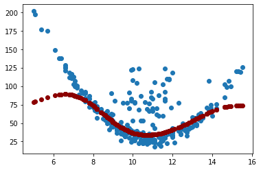
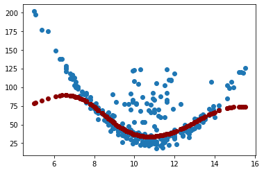
Regresión no lineal:
Kernel: RBF:
svm_reg = SVR(kernel="rbf")
svm_reg.fit(X, y)
y_pred = svm_reg.predict(X)
r2_score(y, y_pred)
0.33146083387157166
mean_squared_error(y, y_pred)
707.1424760452836
plt.scatter(X, y)
plt.scatter(X.values, y_pred, color="darkred")
<matplotlib.collections.PathCollection at 0x1cd4143cb80>
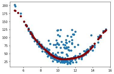
Kernel: Polinómica:
svm_reg = SVR(kernel="poly", degree=4)
svm_reg.fit(X, y)
y_pred = svm_reg.predict(X)
r2_score(y, y_pred)
-0.11184886055676602
mean_squared_error(y, y_pred)
1176.0501045816075
plt.scatter(X, y)
plt.scatter(X.values, y_pred, color="darkred")
<matplotlib.collections.PathCollection at 0x1cd414aea60>
Regularización del modelo:
El mejor modelo fue el del kernel RBF.
Se cambiará el hiperparámetro: epsilon
svm_reg = SVR(kernel="rbf", epsilon=0.5)
svm_reg.fit(X, y)
y_pred = svm_reg.predict(X)
r2_score(y, y_pred)
0.3331817646255232
mean_squared_error(y, y_pred)
705.3221739656027
plt.scatter(X, y)
plt.scatter(X.values, y_pred, color="darkred")
<matplotlib.collections.PathCollection at 0x1cd41521640>
Se cambiará el hiperparámetro: gamma
svm_reg = SVR(kernel="rbf", gamma=0.5)
svm_reg.fit(X, y)
y_pred = svm_reg.predict(X)
r2_score(y, y_pred)
0.30117215778379613
mean_squared_error(y, y_pred)
739.1801044895215
plt.scatter(X, y)
plt.scatter(X.values, y_pred, color="darkred")
<matplotlib.collections.PathCollection at 0x1cd41591820>

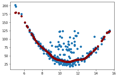
Se cambiará el hiperparámetro: C
svm_reg = SVR(kernel="rbf", C=50)
svm_reg.fit(X, y)
y_pred = svm_reg.predict(X)
r2_score(y, y_pred)
0.5592769445039655
mean_squared_error(y, y_pred)
466.1716298815007
plt.scatter(X, y)
plt.scatter(X.values, y_pred, color="darkred")
<matplotlib.collections.PathCollection at 0x1cd416044c0>
Se cambiarán los hiperparámetros: epsilon, gamma y C.
svm_reg = SVR(kernel="rbf", epsilon=0.5, gamma=0.7, C=50)
svm_reg.fit(X, y)
y_pred = svm_reg.predict(X)
r2_score(y, y_pred)
0.5655477014368502
mean_squared_error(y, y_pred)
459.5387820113037
plt.scatter(X, y)
plt.scatter(X.values, y_pred, color="darkred")
<matplotlib.collections.PathCollection at 0x1cd41666e50>