Práctica - clasificación
import pandas as pd
import numpy as np
import matplotlib.pyplot as plt
from sklearn.preprocessing import StandardScaler
from sklearn.linear_model import LogisticRegression
from sklearn.svm import SVC
from sklearn.tree import DecisionTreeClassifier
from sklearn.metrics import accuracy_score
from matplotlib.colors import ListedColormap
from sklearn import tree
Lectura de datos:
df = pd.read_csv("Social_Network_Ads.csv", sep=",", decimal=".")
print(df.head())
    User ID  Gender  Age  EstimatedSalary  Purchased
0  15624510    Male   19            19000          0
1  15810944    Male   35            20000          0
2  15668575  Female   26            43000          0
3  15603246  Female   27            57000          0
4  15804002    Male   19            76000          0
Información de cada columna de la base de datos y cantidad de valores nulos:
df.info()
<class 'pandas.core.frame.DataFrame'>
RangeIndex: 400 entries, 0 to 399
Data columns (total 5 columns):
 #   Column           Non-Null Count  Dtype
---  ------           --------------  -----
 0   User ID          400 non-null    int64
 1   Gender           400 non-null    object
 2   Age              400 non-null    int64
 3   EstimatedSalary  400 non-null    int64
 4   Purchased        400 non-null    int64
dtypes: int64(4), object(1)
memory usage: 15.8+ KB
Cantidad de distintos elementos por columna:
df.nunique()
User ID            400
Gender               2
Age                 43
EstimatedSalary    117
Purchased            2
dtype: int64
Identificar cada fila como el ID:
df.set_index("User ID", inplace=True)
print(df.head())
          Gender  Age  EstimatedSalary  Purchased
User ID
15624510    Male   19            19000          0
15810944    Male   35            20000          0
15668575  Female   26            43000          0
15603246  Female   27            57000          0
15804002    Male   19            76000          0
Análisis de las variables:
df.hist()
array([[<AxesSubplot:title={'center':'Age'}>,
        <AxesSubplot:title={'center':'EstimatedSalary'}>],
       [<AxesSubplot:title={'center':'Purchased'}>, <AxesSubplot:>]],
      dtype=object)
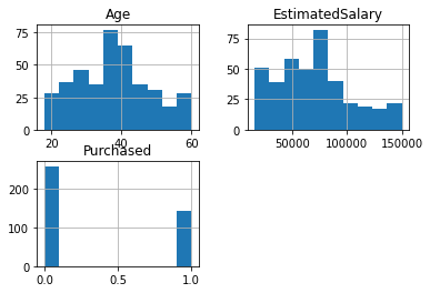
print(df.describe())
              Age  EstimatedSalary   Purchased
count  400.000000       400.000000  400.000000
mean    37.655000     69742.500000    0.357500
std     10.482877     34096.960282    0.479864
min     18.000000     15000.000000    0.000000
25%     29.750000     43000.000000    0.000000
50%     37.000000     70000.000000    0.000000
75%     46.000000     88000.000000    1.000000
max     60.000000    150000.000000    1.000000
Transformación de atributos categóricos:
df.value_counts("Gender")
Gender
Female    204
Male      196
dtype: int64
from sklearn.preprocessing import LabelEncoder
gender_encoder = LabelEncoder()
df["Gender"] = gender_encoder.fit_transform(df["Gender"])
print(df.head())
          Gender  Age  EstimatedSalary  Purchased
User ID
15624510       1   19            19000          0
15810944       1   35            20000          0
15668575       0   26            43000          0
15603246       0   27            57000          0
15804002       1   19            76000          0
Conjunto de datos para el modelo:
X = pd.concat([df[["Gender", "Age", "EstimatedSalary"]]], axis=1)
print(X)
          Gender  Age  EstimatedSalary
User ID
15624510       1   19            19000
15810944       1   35            20000
15668575       0   26            43000
15603246       0   27            57000
15804002       1   19            76000
...          ...  ...              ...
15691863       0   46            41000
15706071       1   51            23000
15654296       0   50            20000
15755018       1   36            33000
15594041       0   49            36000

[400 rows x 3 columns]
y = df["Purchased"]
print(y)
User ID
15624510    0
15810944    0
15668575    0
15603246    0
15804002    0
           ..
15691863    1
15706071    1
15654296    1
15755018    0
15594041    1
Name: Purchased, Length: 400, dtype: int64
División del conjunto de datos:
len(X)
400
from sklearn.model_selection import train_test_split
X_train, X_test, y_train, y_test = train_test_split(X, y, test_size=0.2, random_state=0)
Escalado de variables:
from sklearn.preprocessing import StandardScaler
sc = StandardScaler()
sc.fit(X_train)
X_train_std = sc.transform(X_train)
X_test_std = sc.transform(X_test)
print(X_train_std[:10])
[[ 1.02532046  1.92295008  2.14601566]
 [-0.97530483  2.02016082  0.3787193 ]
 [-0.97530483 -1.3822153  -0.4324987 ]
 [-0.97530483 -1.18779381 -1.01194013]
 [-0.97530483  1.92295008 -0.92502392]
 [-0.97530483  0.36757813  0.29180308]
 [-0.97530483  0.17315664  0.14694273]
 [ 1.02532046  2.02016082  1.74040666]
 [-0.97530483  0.75642112 -0.83810771]
 [-0.97530483  0.27036739 -0.28763835]]
print(X_test_std[:10])
[[ 1.02532046 -0.79895082  0.49460758]
 [-0.97530483 -0.02126485 -0.57735906]
 [ 1.02532046 -0.31289709  0.14694273]
 [-0.97530483 -0.79895082  0.26283101]
 [-0.97530483 -0.31289709 -0.57735906]
 [ 1.02532046 -1.09058306 -1.44652121]
 [-0.97530483 -0.70174008 -1.59138156]
 [ 1.02532046 -0.21568634  2.14601566]
 [-0.97530483 -1.96547978 -0.05586178]
 [ 1.02532046  0.85363187 -0.78016356]]
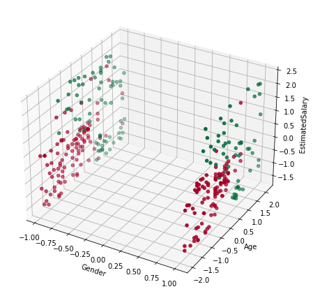
Visualización de los datos:
from mpl_toolkits import mplot3d
fig = plt.figure(figsize=(8, 6))
axes = plt.axes(projection="3d")
axes.scatter3D(
    X_train_std[:, 0],
    X_train_std[:, 1],
    X_train_std[:, 2],
    c=y_train,
    cmap=plt.cm.RdYlGn,
)
axes.set_xlabel("Gender")
axes.set_ylabel("Age")
axes.set_zlabel("EstimatedSalary")
plt.tight_layout()
plt.show()
Ajuste de los modelos de clasificación:
Conjunto de entrenamiento:
log_reg = LogisticRegression()
log_reg.fit(X_train_std, y_train)
y_pred = log_reg.predict(X_train_std)
accuracy_score(y_train, y_pred)
0.825
Conjunto de prueba:
y_pred = log_reg.predict(X_test_std)
accuracy_score(y_test, y_pred)
0.9125
SVM: kernel lineal:
Conjunto de entrenamiento:
clf = SVC(kernel="linear", random_state=0)
clf.fit(X_train_std, y_train)
y_pred = clf.predict(X_train_std)
accuracy_score(y_train, y_pred)
0.821875
Conjunto de prueba:
y_pred = clf.predict(X_test_std)
accuracy_score(y_test, y_pred)
0.9125
SVM: kernel RBF:
Conjunto de entrenamiento:
clf = SVC(kernel="rbf", random_state=0)
clf.fit(X_train_std, y_train)
y_pred = clf.predict(X_train_std)
accuracy_score(y_train, y_pred)
0.896875
Conjunto de prueba:
y_pred = clf.predict(X_test_std)
accuracy_score(y_test, y_pred)
0.95
Árboles de clasificación:
Conjunto de entrenamiento:
clf = DecisionTreeClassifier(random_state=0)
clf.fit(X_train_std, y_train)
y_pred = clf.predict(X_train_std)
accuracy_score(y_train, y_pred)
1.0
Conjunto de prueba:
y_pred = clf.predict(X_test_std)
accuracy_score(y_test, y_pred)
0.9
Regularización del árbol:
Cambiando max_depth.
Conjunto de entrenamiento:
clf = DecisionTreeClassifier(max_depth=3, random_state=0)
clf.fit(X_train_std, y_train)
y_pred = clf.predict(X_train_std)
accuracy_score(y_train, y_pred)
0.9125
Conjunto de prueba:
y_pred = clf.predict(X_test_std)
accuracy_score(y_test, y_pred)
0.95