Árboles de decisión - Regresión - código

Importar librerías:

import pandas as pd
import numpy as np
import matplotlib.pyplot as plt

Importar datos:

df = pd.read_csv("regresion.csv", sep=";", decimal=",")
print(df.head())

      X     y
0   9.0  44.7
1  10.1  78.0
2  11.6  83.0
3   9.1  80.0
4   9.7  77.0

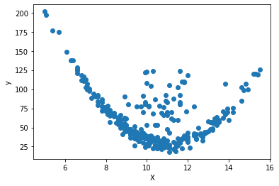
Visualización de los datos:

plt.scatter(df["X"], df["y"])
plt.xlabel("X")
plt.ylabel("y")

Text(0, 0.5, 'y')

Ajuste del modelo:

X = df[["X"]]
print(X.head())

      X
0   9.0
1  10.1
2  11.6
3   9.1
4   9.7

y = df["y"]
print(y.head())

0    44.7
1    78.0
2    83.0
3    80.0
4    77.0
Name: y, dtype: float64

from sklearn.tree import DecisionTreeRegressor

tree_reg = DecisionTreeRegressor(random_state=0)

tree_reg.fit(X, y)

DecisionTreeRegressor(random_state=0)

y_pred = tree_reg.predict(X)

Evaluación del desempeño:

from sklearn.metrics import r2_score, mean_squared_error

r2_score(y, y_pred)

0.7064753910416934

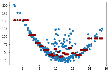
mean_squared_error(y, y_pred)

310.4735358453583

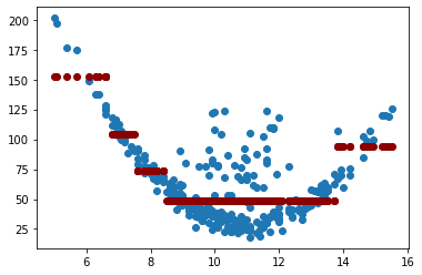
plt.scatter(X, y)
plt.scatter(X.values, y_pred, color="darkred")

<matplotlib.collections.PathCollection at 0x1ccec1a5f70>

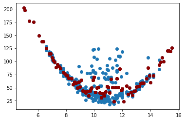
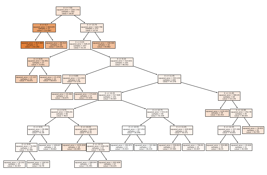
Aunque no se obtiene un modelo con un \(R^2\) igual a 1 o un MSE igual a 0, se puede ver en el gráfico que el modelo trata de sobreajustarse a la estructura de los datos. Con la visualización del árbol podemos concluir también que el modelo está sobreajustado.

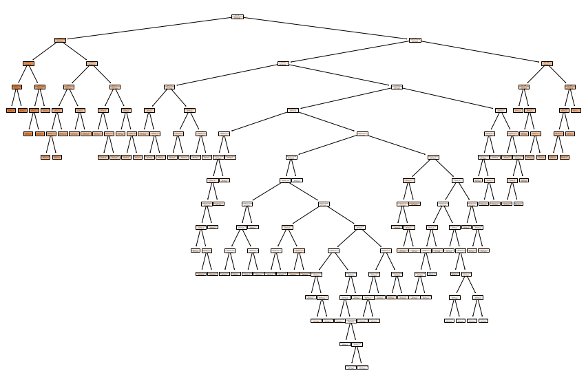
Visualización del árbol:

from sklearn import tree

feature_names = df.columns.values[0:2]
plt.figure(figsize=(15, 10))
tree.plot_tree(tree_reg, feature_names=feature_names, filled=True);

Regularización del modelo:

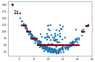
Cambiaremos min_samples_leaf. Entre más alto el valor asignado menos es el sobreajuste.

tree_reg = DecisionTreeRegressor(random_state=0, min_samples_leaf=10)

tree_reg.fit(X, y)
y_pred = tree_reg.predict(X)

r2_score(y, y_pred)

0.6232298523322551

mean_squared_error(y, y_pred)

398.52590337322766

plt.scatter(X, y)
plt.scatter(X.values, y_pred, color="darkred")

<matplotlib.collections.PathCollection at 0x1ccec6cfdf0>

feature_names = df.columns.values[0:2]
plt.figure(figsize=(15, 10))
tree.plot_tree(tree_reg, feature_names=feature_names, filled=True);

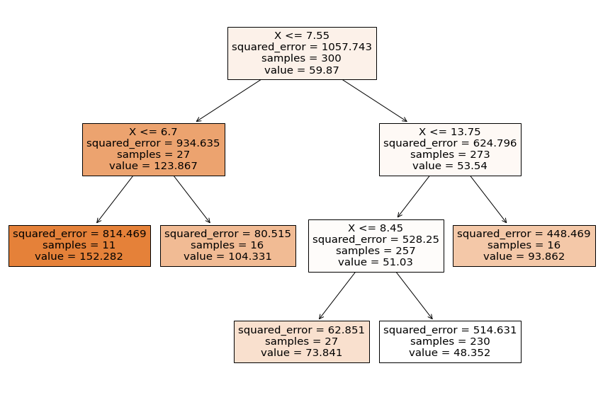
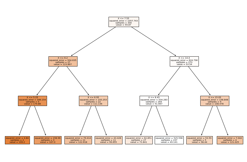
Cambiaremos max_depth. Entre más bajo el valor asignado menos es el sobreajuste.

tree_reg = DecisionTreeRegressor(random_state=0, max_depth=3)

tree_reg.fit(X, y)
y_pred = tree_reg.predict(X)

r2_score(y, y_pred)

0.5953725060234119

mean_squared_error(y, y_pred)

427.991810298271

plt.scatter(X, y)
plt.scatter(X.values, y_pred, color="darkred")

<matplotlib.collections.PathCollection at 0x1ccec391340>

feature_names = df.columns.values[0:2]
plt.figure(figsize=(15, 10))
tree.plot_tree(tree_reg, feature_names=feature_names, filled=True);

Cambiaremos min_samples_leaf y max_depth.

tree_reg = DecisionTreeRegressor(random_state=0, min_samples_leaf=10, max_depth=3)

tree_reg.fit(X, y)
y_pred = tree_reg.predict(X)

r2_score(y, y_pred)

0.5667346543636781

mean_squared_error(y, y_pred)

458.2832911228835

plt.scatter(X, y)
plt.scatter(X.values, y_pred, color="darkred")

<matplotlib.collections.PathCollection at 0x1ccec2d64c0>

feature_names = df.columns.values[0:2]
plt.figure(figsize=(15, 10))
tree.plot_tree(tree_reg, feature_names=feature_names, filled=True);